JEPA-v0: a self-supervised audio encoder for real-time speech translation

Why audio encoders matter

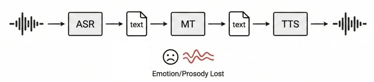
Imagine you’re on a video call with a colleague in Tokyo. She’s explaining, with rising excitement in her voice, why a project deadline needs to move. You don’t speak Japanese, so a translation system kicks in. That system transcribes her speech to text, translates the text, and reads it back with a robotic voice. You might get the words, but you lose the urgency, the sentiment, the person. That’s the fundamental problem with traditional translation models based on cascaded translation pipelines. The cascade pipeline of ASR → MT → TTS treats audio as a container for text. It cracks open the container, throws the container away, translates the text inside, and builds a new container from scratch. Everything that made the original speech human, like pitch and rhythm, gets discarded at step one and cannot be naturally recovered.

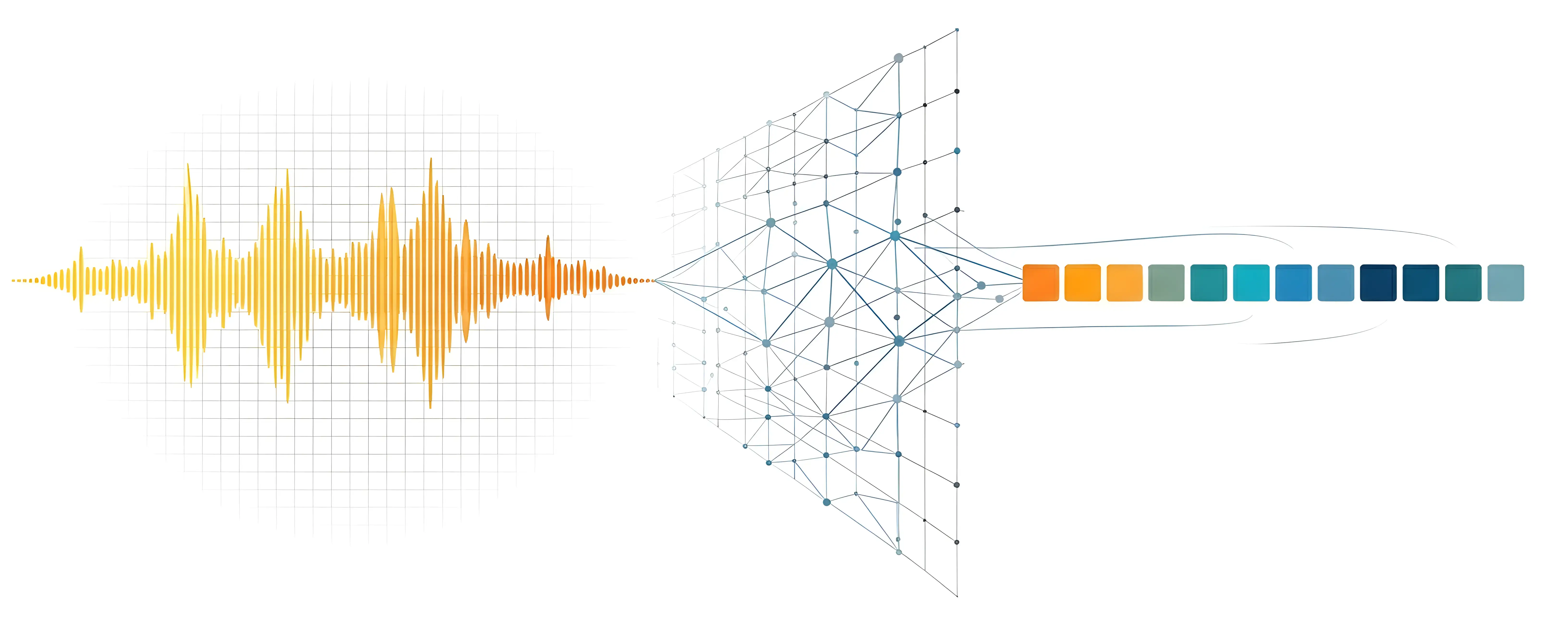
A better approach works directly with rich audio representations that carry both what was said and how it was said. Systems like Meta’s SeamlessStreaming and Kyutai’s Hibiki point in this direction: encode the source speech into a representation that preserves meaning alongside paralinguistic information, then decode that representation into the target language while keeping the speaker’s characteristics intact.

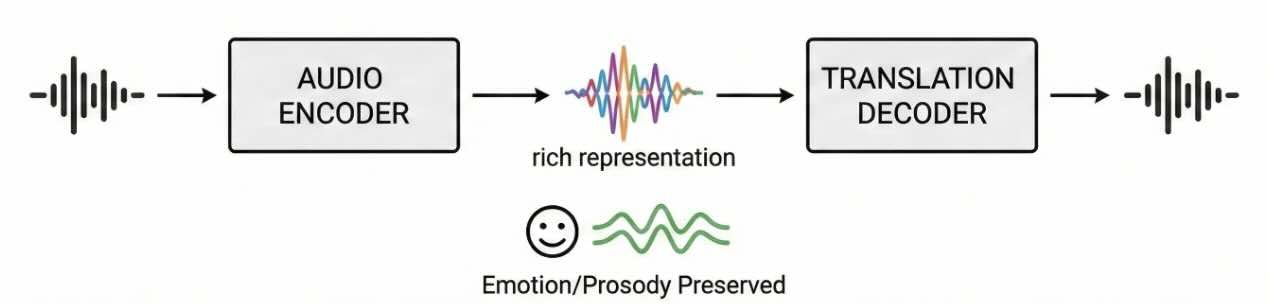
A core component for the speech-to-speech approach is the audio encoder, which takes raw audio and compresses it into a useful representation. If the encoder strips out emotion and prosody (like a transcription model does), no downstream translator can recover them. If the encoder preserves them, everything downstream has a better chance. The quality of this encoder determines the ceiling of everything downstream.

That’s what JEPA-v0 is: our attempt to build an audio encoder whose representations are rich enough to power real-time speech-to-speech translation.

Why self-supervised? The labeled data bottleneck

Consider what you’d need to train a supervised multilingual audio encoder from scratch. You’d want parallel speech data: the same utterance spoken in English, Portuguese, Japanese, Arabic, Mandarin, and dozens more languages. You’d want speaker labels, emotion annotations, prosody markers. Datasets like this barely exist, and where they do, they cover a handful of language pairs in controlled recording conditions.

Supervised speech encoders like Whisper sidestep this by training on a massive but narrow task: transcription. Whisper saw 680k hours of labeled speech-text pairs, and it learned extremely good representations for turning speech into text. But its representations are optimized for lexical content, not for the paralinguistic features a translation system needs.

Self-supervised learning flips the script. Instead of telling the model what to learn from the data (transcribe this, classify that), you let the model discover structure on its own. The model learns from the raw audio itself without anyone labeling anything. This is the same insight that made BERT and GPT transformative for text: pre-train a general representation from unlabeled data, then let downstream models specialize.

For JEPA-v0, this means we can train on millions of audio samples spanning speech in multiple languages, environmental sounds, and music, all without needing a single label. The encoder learns a rich structure to represent the data: phonetic patterns, speaker characteristics, emotional valence, rhythmic structure, acoustic events.

Learning by predicting what you can’t see

Self-supervised learning for audio has two dominant approaches, each with a clear analogy that makes the tradeoff intuitive.

The jigsaw puzzle approach: masked reconstruction

Imagine someone gives you a spectrogram of an audio sentence. They cover 40% of it with gray blocks and ask you to fill in the missing pieces. That’s masked reconstruction, used by models like AudioMAE.

To fill in the blanks, you need to understand a lot about audio: what speech sounds like, how harmonics relate to fundamentals, how consonants transition into vowels. The model does learn useful representations this way. But there is a catch: it has to predict exact spectrogram values. It spends a lot of its memory on remembering the exact room reverberation, microphone quirks, and other noise that aren’t important for the downstream translation model. It shifts the model’s task from learning representations to performing reconstruction.

The matching game approach: contrastive learning

Now imagine a different game. Someone takes an audio clip, creates two distorted copies (one pitch-shifted up, one with added background noise), and asks: “are these the same original clip?” That’s contrastive learning, used by models like wav2vec 2.0 and BYOL.

The model learns by pulling representations of the same audio together and pushing different audios apart. It works well, but the distortions (called augmentations) are designed by humans, and they implicitly decide what the model treats as “irrelevant variation.” If you always augment with pitch shifts, the model learns to ignore pitch, but this might be what you don’t want for a translation encoder that needs to preserve the speaker’s intonation.

JEPA: predict the meaning, not the details

JEPA (Joint-Embedding Predictive Architecture) offers a third path that avoids both problems. The idea, proposed by Yann LeCun in his 2022 position paper “A Path Towards Autonomous Machine Intelligence”, is as elegant as it is counterintuitive: predict the representation of the hidden parts, not the hidden parts themselves.

Here’s the difference. In masked reconstruction, if you hide a region containing a dog bark, the model must predict the exact spectral shape of that bark. In JEPA, the model only needs to predict what another encoder thinks about that region, an abstract summary that captures “there’s a dog bark here” without committing to the acoustic details. This forces the model to focus on what matters: the semantic and structural content of audio. For a translation encoder, this is the ideal tradeoff: learn everything about the speech content, the speaker’s characteristics, and the emotional tone, while ignoring the irrelevant specifics of a particular microphone or room.

How Audio JEPA works

Audio JEPA has three components that work together during training. To make this concrete, let’s walk through what happens with a single 10-second audio clip.

Context encoder

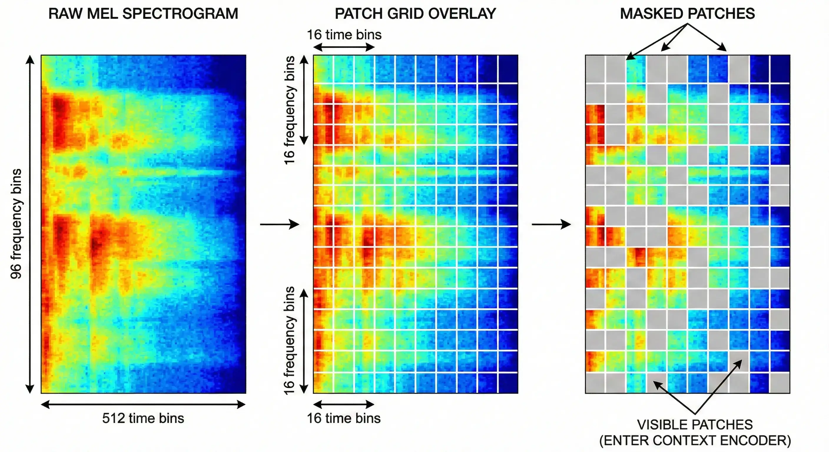
First, the raw audio waveform gets converted into a log-mel spectrogram, a heatmap showing which frequencies are present at each moment in time. Our spectrogram has 512 time steps and 96 frequency bins, giving us a 512×96 image.

This image gets chopped into small, non-overlapping patches of 16×16 pixels, like tiles on a mosaic floor. That gives us 32 patches along time × 6 patches along frequency = 192 patches total. Each patch is projected into a 768-dimensional vector (its “embedding”) and receives a positional encoding that tells the transformer where on the time-frequency grid it sits.

A multi-block masking strategy determines which patches the context encoder sees and which ones it must predict. First, three prediction blocks are sampled, each covering 15–20% of the patch grid, with randomized aspect ratios so the model can’t learn to expect a fixed shape. These blocks can overlap each other, so together they select roughly 35–50% of the grid as prediction targets. After that, a large context block (80–100% of the grid) is sampled, and the prediction regions are subtracted from it. The result is that the context encoder typically sees around 40–55% of the patches.

The context encoder is a Vision Transformer (ViT-Base): 12 transformer layers, 12 attention heads, 768 hidden dimensions, roughly 86 million parameters. It processes those ~155 visible patch embeddings and produces a 768-dimensional representation for each.

Think of the context encoder as a reader with missing pages. It builds the best understanding it can from incomplete information, and it never knows in advance which pages will be missing, so it has to learn representations that are robust regardless of what’s hidden.

Target encoder

The target encoder has the same architecture as the context encoder, but it sees all 192 patches with nothing masked. It processes the full spectrogram and produces a 768-dimensional representation for every patch position.

After the target encoder runs, its output is indexed at the masked positions (the ones the context encoder didn’t see) to extract the representations the predictor must match. These target representations are the “answers” for the prediction task. The target encoder’s weights aren’t trained by gradient descent. Instead, they’re an exponential moving average (EMA) of the context encoder’s weights. After each training step, the target encoder’s weights get nudged slightly toward the context encoder’s:

θ_target ← τ · θ_target + (1 − τ) · θ_context

where τ (the momentum) starts at 0.996 and slowly approaches 1.0. Think of the target encoder as a teacher who changes their mind very slowly. When the student (context encoder) rapidly adjusts its understanding, the teacher stays mostly stable, providing consistent learning targets. This slow evolution matters because without it, the system collapses (more on that soon).

Predictor

The predictor takes the context encoder’s output, representations of the ~155 visible patches, and must predict what the target encoder produced at the ~37 masked positions. It knows where the gaps are (via positional encodings for both visible and masked positions) but has never seen their content.

The predictor first projects the context embeddings from 768 down to 384 dimensions (a dimensional bottleneck). It then creates learnable “mask tokens” (placeholder vectors) for each masked position and concatenates them with the projected context embeddings. A 6-layer transformer processes this combined sequence, allowing the mask tokens to attend to the context tokens and gather the information they need. Finally, only the mask token outputs are extracted and projected back up to 768 dimensions for comparison with the target.

Because the predictor can only reconstruct masked positions from the visible ones, the context encoder is pressured to spread useful, predictive information across all of its output embeddings. If any visible patch carries a weak representation, the predictor will fail whenever nearby patches are masked. The training loss is the distance between the predictor’s output and the target encoder’s representation, computed after both are normalized to unit length (L2 normalization). Minimizing this normalized MSE is equivalent to maximizing the cosine similarity between the two representations. The model learns to match the direction of embeddings (their semantic meaning), not their magnitude.

Why this doesn’t collapse

If the context encoder, target encoder, and predictor all output the same constant vector for every input, the loss would be zero. The model would have “learned” nothing useful, but it would have minimized the training objective. This is called representational collapse, and it’s the main failure mode of self-supervised methods without negative examples. JEPA prevents collapse through three mechanisms:

• The stop-gradient on the target: Gradients only flow through the predictor and context encoder, never through the target encoder. The target encoder can’t adapt to make prediction easier. It just slowly follows the context encoder via EMA.
• The EMA momentum: Because the target changes slowly while the context encoder updates rapidly, there’s always a gap between them. The context encoder is always chasing a moving target it can never fully reach, which keeps it from settling into a trivial solution.
• The predictor bottleneck: By compressing to 384 dimensions, the predictor can’t simply memorize or copy the input. It has to capture predictive structure, patterns that generalize across different masked regions.

Ponce et al. (ICLR 2026) proved something surprising about this: EMA-based training dynamics like JEPA’s don’t optimize any smooth mathematical function, yet they provably converge to useful, non-collapsed representations. The equilibria are asymptotically stable, meaning the system naturally falls into states where the representations are informative.

What the representations capture

We evaluated JEPA-v0 on the XARES benchmark, which tests frozen audio encoders across classification and understanding tasks spanning speech, environmental sound, and music. We compare against three strong baselines: Audio-JEPA, a self-supervised audio encoder; Whisper, a supervised speech encoder trained on 680k hours of labeled data; and Mimi, Kyutai’s neural audio codec.

Task	JEPA-v0	Audio-JEPA	Whisper	Mimi
Spoofing detection	0.927	0.939	0.946	0.962
Music captioning (SongDescriber)	0.481	0.445	0.447	0.473
General captioning (MeCat)	0.478	0.490	0.625	0.583
Vocal sound classification	0.795	0.401	0.866	0.907
Emotion recognition (CREMA-D)	0.456	0.383	0.506	0.580
Keyword spotting (SpeechCommands)	0.091	0.052	0.707	0.678
Language identification	0.078	0.044	0.829	0.540
Intent classification	0.155	0.104	0.823	0.983
Speech recognition (LibriSpeech)	0.000	0.000	0.375	0.637
Speech recognition (AISHELL-1)	0.000	0.000	0.359	0.157

JEPA-v0 matches baseline models when it comes to spotting fake audio. It scored 0.927, while Whisper scored 0.946 and Mimi scored 0.962. This task checks if a human throat and mouth actually made the sound. The encoder spends a lot of its processing power on speaker details like the shape of the vocal tract, the pitch, and specific spectral data. The model currently struggles when it has to attach meaning to those sounds. For example, in general captioning, it scored 0.478 compared to Whisper’s 0.625 and Mimi’s 0.583, and in speech recognition it scored 0.000 compared to Whisper’s 0.375 and Mimi’s 0.637.

Let’s take a look at the embeddings for a few examples from each dataset.

LibriSpeech

LibriSpeech is a corpus of approximately 1000 hours of read English speech derived from public domain audiobooks. The dataset is widely used for training and evaluating automatic speech recognition (ASR) systems, and it is also valuable for research in speech processing, speaker recognition, and audio understanding. Let’s take a randomly selected example from the LibriSpeech dataset and visualize its embeddings.

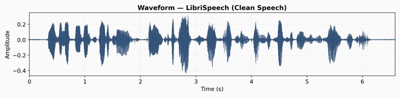
To visualize the embeddings, let’s use a latent space trajectory plot. The animation shows the evolution of the audio embedding as the audio is “played” in the spectrogram. The latent space trajectory uses PCA to project the embedding into a 2D space. The variation over time displays how consistent the embeddings learned by the model capture differences in the audio signal.

The LibriSpeech latent trajectory shows a massive information bottleneck. The first two principal components cover 78.6% of the embedding variance, which means the model has reduced almost all its data into a tiny space. The movement seems to capture weak phonetic patterns and mostly changes over volume and sound texture.

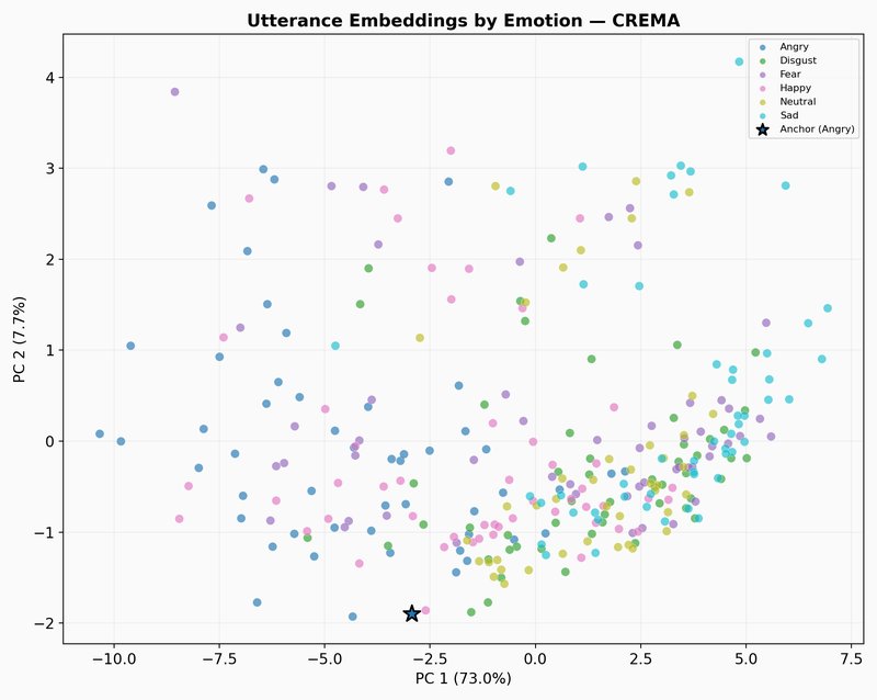
CREMA-D

CREMA-D is a dataset of emotional speech recordings from 91 actors, featuring a range of emotions, intensities, and speaking styles. It is widely used for research in emotion recognition, speech processing, and affective computing. Again, let’s take a randomly selected example from the CREMA-D dataset and visualize its embeddings.

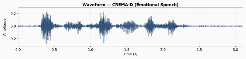
The CREMA-D latent trajectory path is different than LibriSpeech. Instead of one dense cluster, the path jumps across a wider area. These jumps match the sharp changes in the spectrogram, like sudden bursts of energy or shifts in pitch that happen in emotional acting. The model captures these broad acoustic patterns, which is why JEPA-v0 gets a 0.456 score on CREMA-D emotion recognition. It tracks volume, pitch range, and speed because those things relate to emotional categories.

The illustration below shows what happens when we zoom out from the selected clip to other randomly selected samples from the CREMA-D dataset. Each dot is one emotional speech track, mean-pooled into a single embedding and colored by emotion labels.

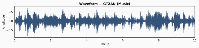
GTZAN

GTZAN is a dataset of audio recordings of music from 10 different genres, including blues, classical, disco, jazz, metal, pop, rock, and more. It is widely used for research in music information retrieval, genre classification, and audio understanding. Let’s take a randomly selected example from the GTZAN dataset.

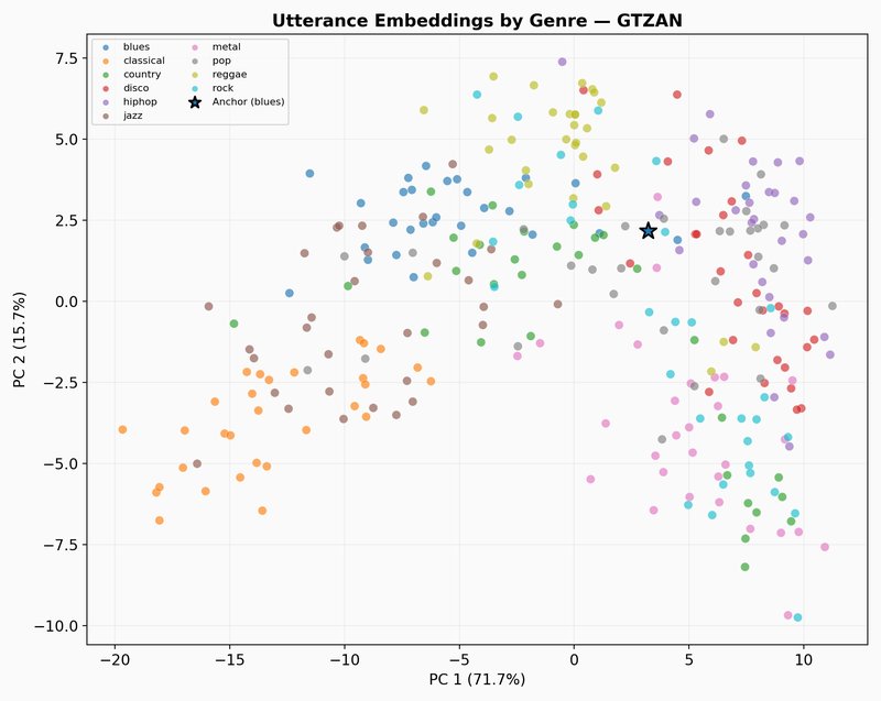
The GTZAN latent trajectory shows a completely different dynamics. The first two components explain 59.2% of the variance, which is a 20% drop compared to the speech datasets. Instead of sticking to tight clusters, the path fills the entire plane. This higher dimensionality shows that the model is learning how to capture the texture of tone, harmony and rhythm, and helps JEPA-v0 to get a competitive score of 0.481 for music captioning.

The scatter plot below shows what happens when we zoom out from the selected clip to other randomly selected samples from the GTZAN dataset. Each dot is one music track, mean-pooled into a single embedding and colored by genre.

The path forward: from encoder to translator

Our JEPA model is one building block in the larger system we’re building at Pinch. The encoder provides front-end representations that a translation model consumes. The current model excels at distinguishing kinds of sounds (speech, music, noise) but has difficulty modeling phonemic sequences and speech meaning.

The XARES benchmark results and latent trajectory visualizations give us a picture of what JEPA-v0 captures and what it misses. The encoder picks up broad acoustic structure well: timbral qualities, spectral texture, and emotional shifts in speech. The CREMA-D trajectories show the model tracking pitch and energy changes that correlate with emotional categories, and the GTZAN trajectories show it spreading representations across a rich space that distinguishes musical texture. But when the task requires mapping audio to linguistic content, the encoder falls short. The LibriSpeech trajectory confirms this visually: most of the embedding variance collapses into a narrow region, suggesting the model treats different phonemes as near-identical. The encoder also does not align meaning across languages, as semantically equivalent utterances in different languages occupy separate regions of the embedding space, and therefore cross-lingual mapping will need to come from a downstream model or from changes to the training objective.

The most direct bottleneck is the 32-frame output for a 10-second clip. We can increase temporal resolution by reducing the patch size, increasing the spectrogram resolution, or using hierarchical representations at multiple time scales. The GTZAN latent trajectory hints at what’s possible. Music’s rapid frame-to-frame variation forces the encoder into higher-dimensional, more informative representations. Speech should demand the same, if the temporal resolution allows it.

We also need to preserve frequency structure. Currently, we average over the frequency axis to produce 1D frame-level embeddings, which collapses information that distinguishes vowels from consonants (formant structure), pitch (fundamental frequency), and timbral details. Retaining a 2D output or using frequency-aware pooling strategies could keep these cues, and they’re needed for high-quality translation.

Finally, we need to connect the encoder to a translation decoder. The FSQ output feeds directly into autoregressive sequence models. We’re testing whether JEPA representations can drive speech-to-speech translation while preserving the speaker characteristics that text-based pipelines discard. That’s where the encoder faces its real test: not classification benchmarks, but whether a translated voice still sounds like the original speaker.

References

LeCun, “A Path Towards Autonomous Machine Intelligence” (2022). The position paper that introduced JEPA as a blueprint for world models.

Assran et al., “Self-Supervised Learning from Images with a Joint-Embedding Predictive Architecture” (CVPR 2023). The first practical JEPA implementation, applied to vision.

Tuncay et al., “Audio-JEPA: Joint-Embedding Predictive Architecture for Audio Representation Learning” (ICME 2025). The methodological foundation for Pinch-JEPA; adapts I-JEPA to audio spectrograms.

Ioannides et al., “JEPA as a Neural Tokenizer” (2024). Combines JEPA with FSQ for speech tokenization at very low bitrates.

Mentzer et al., “Finite Scalar Quantization: VQ-VAE Made Simple” (ICLR 2024). The quantization method we use to discretize encoder output.

Zhang et al., “X-ARES: A Comprehensive Framework for Assessing Audio Encoder Performance” (2025). The evaluation framework we used to benchmark Pinch-JEPA.

Ponce et al., “Dual Perspectives on Non-Contrastive Self-Supervised Learning” (ICLR 2026). Proves that EMA-based methods like JEPA converge to useful representations despite not optimizing any smooth function.